Graph Embeddings

Due to their nature, graphs can be analyzed at different levels of granularity: at the node, edge, and graph level (the whole graph), as depicted in the following figure. For each of those levels, different problems could be faced and, as a consequence, specific algorithms should be used.

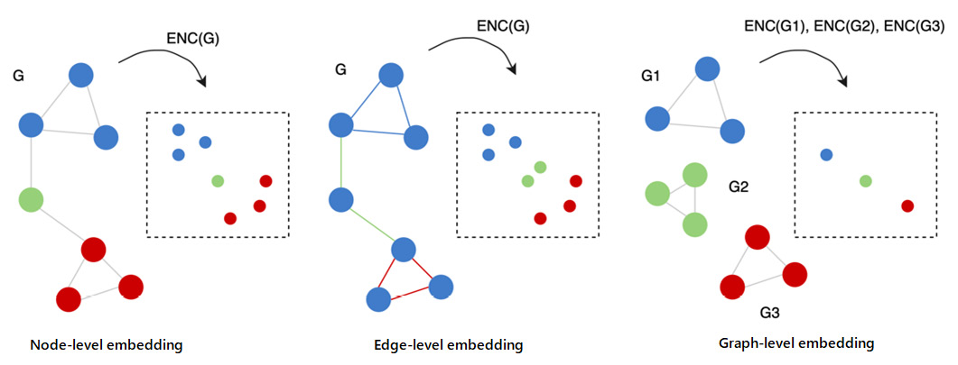
Visual representation of the three different levels of granularity in graphs

The first, and most straightforward, way of creating features capable of representing structural information from graphs is the extraction of certain statistics. For instance, a graph could be represented by its degree distribution, efficiency, and other metrics.

A more complex procedure consists of applying specific kernel functions or, in other cases, engineering-specific features that are capable of incorporating the desired properties into the final machine learning model. However, as you can imagine, this process could be really time-consuming and, in certain cases, the features used in the model could represent just a subset of the information that is really needed to get the best performance for the final model.

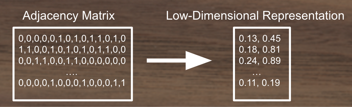
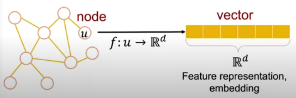
Converting Adjacency Matrices to low-dimensional continuous vector spaces.

In the last decade, a lot of work has been done in order to define new approaches for creating meaningful and compact representations of graphs. The general idea behind all these approaches is to create algorithms capable of learning a good representation of the original dataset such that geometric relationships in the new space reflect the structure of the original graph. We usually call the process of learning a good representation of a given graph representation learning or network embedding.

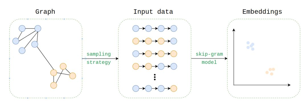
Example of a workflow for a network embedding algorithm

The generalized network embedding problem

Network embedding is the task that aims at learning a mapping function from a discrete graph to a continuous domain. Formally, given a graph $G = (V, E)$ with weighted adjacency matrix $W \in \mathbb{R}^{|V|×|V|}$, the goal is to learn low-dimensional vector representations ${Z_i}_{\{i \in V\}}$ (embeddings) for nodes in the graph ${v_i}_{\{i \in V\}}$, such that important graph properties (e.g. local or global structure) are preserved in the embedding space. For instance, if two nodes have similar connections in the original graph, their learned vector representations should be close. Let $Z \in \mathbb{R}^{|V|×d}$ denote the node embedding matrix. In practice, we often want low-dimensional embeddings ($d \ll |V|$) for scalability purposes. That is, network embedding can be viewed as a dimensionality reduction technique for graph structured data, where the input data is defined on a non-Euclidean, high-dimensional, discrete domain.

Graph level embedding

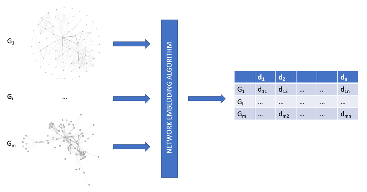
Given a dataset with m different graphs, the task is to build a machine learning algorithm capable of classifying a graph into the right class. We can then see this problem as a classification problem, where the dataset is defined by a list of pairs, $*<G_i,y_i>*$, where $*G_i*$ is a graph and $*y_i*$ is the class the graph belongs to.

Representation learning (network embedding) is the task that aims to learn a mapping function $f:G \to \mathbb{R}^n$, from a discrete graph to a continuous domain. Function $f$ will be capable of performing a low-dimensional vector representation such that the properties (local and global) of graph $G$ are preserved.

Node-level embedding

Given a (possibly large) graph $G = (V,E)$, the goal is to classify each vertex $v \in V$ into the right class. In this setting, the dataset includes $*G*$ and a list of pairs, $*<v_i,y_i>*$, where $*v_i*$ is a node of graph $*G*$ and $*y_i*$ is the class to which the node belongs. In this case, the mapping function would be $f:V \to \mathbb{R}^n$.

The goal of node embedding is "efficient task-independent feature-learning for machine learning with graphs".

Edge level embedding

Given a (possibly large) graph $G = (V,E)$, the goal is to classify each edge $e \in E$, into the right class. In this setting, the dataset includes $*G*$ and a list of pairs, $*<e_i,y_i>*$, where $*e_i*$ is an edge of graph $*G*$ and $*y_i*$ is the class to which the edge belongs. Another typical task for this level of granularity is link prediction, the problem of predicting the existence of a link between two existing nodes in a graph. In this case, the mapping function would be $f:E \to \mathbb{R}^n$.

Encoder and Decoder

Every graph, node, or edge embedding method can be described by two fundamental components, named the encoder and the decoder. The encoder (ENC) maps the input into the embedding space, while the decoder (DEC) decodes structural information about the graph from the learned embedding. It follows an intuitive idea: if we are able to encode a graph such that the decoder is able to retrieve all the necessary information, then the embedding must contain a compressed version of all this information and can be used to downstream machine learning tasks:

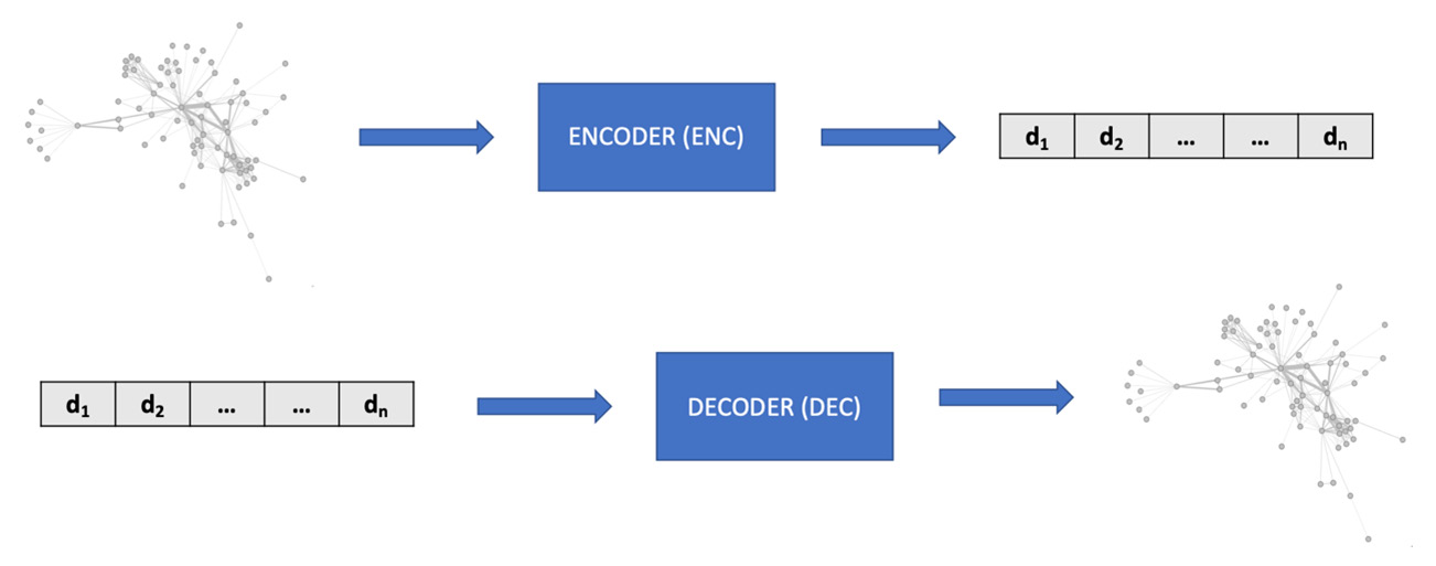
Generalized encoder (ENC) and decoder (DEC) architecture for embedding algorithms

Categorization of embedding algorithms

Shallow embedding methods

These methods are able to learn and return only the embedding values for the learned input data. Node2Vec, Edge2Vec, and Graph2Vec, which we previously discussed, are examples of shallow embedding methods. Indeed, they can only return a vectorial representation of the data they learned during the fit procedure. It is not possible to obtain the embedding vector for unseen data.

Graph autoencoding methods

These methods do not simply learn how to map the input graphs in vectors; they learn a more general mapping function, capable of also generating the embedding vector for unseen instances.

Neighborhood aggregation methods

These algorithms can be used to extract embeddings at the graph level, where nodes are labeled with some properties. Moreover, as for the graph autoencoding methods, the algorithms belonging to this class are able to learn a general mapping function, also capable of generating the embedding vector for unseen instances. A nice property of those algorithms is the possibility to build an embedding space where not only the internal structure of the graph is taken into account but also some external information, defined as properties of its nodes. For instance, with this method, we can have an embedding space capable of identifying, at the same time, graphs with similar structures and different properties on nodes.

Graph regularization methods

Methods based on graph regularization are slightly different from the ones listed in the preceding points. Here, we do not have a graph as input. Instead, the objective is to learn from a set of features by exploiting their "interaction" to regularize the process. In more detail, a graph can be constructed from the features by considering feature similarities. The main idea is based on the assumption that nearby nodes in a graph are likely to have the same labels. Therefore, the loss function is designed to constrain the labels to be consistent with the graph structure. For example, regularization might constrain neighboring nodes to share similar embeddings, in terms of their distance in the L2 norm. For this reason, the encoder only uses X node features as input.

Graph neural networks

GNNs are deep learning methods that work on graph-structured data. This family of methods is also known as geometric deep learning and is gaining increasing interest in a variety of applications, including social network analysis and computer graphics. The original formulation of GNN was proposed by Scarselli et al. back in 2009. It relies on the fact that each node can be described by its features and its neighborhood. Information coming from the neighborhood (which represents the concept of locality in the graph domain) can be aggregated and used to compute more complex and high-level features.

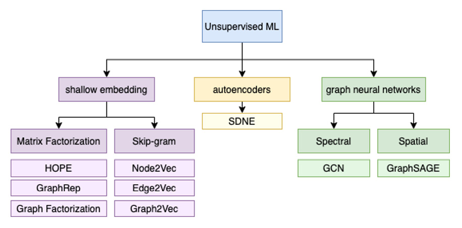
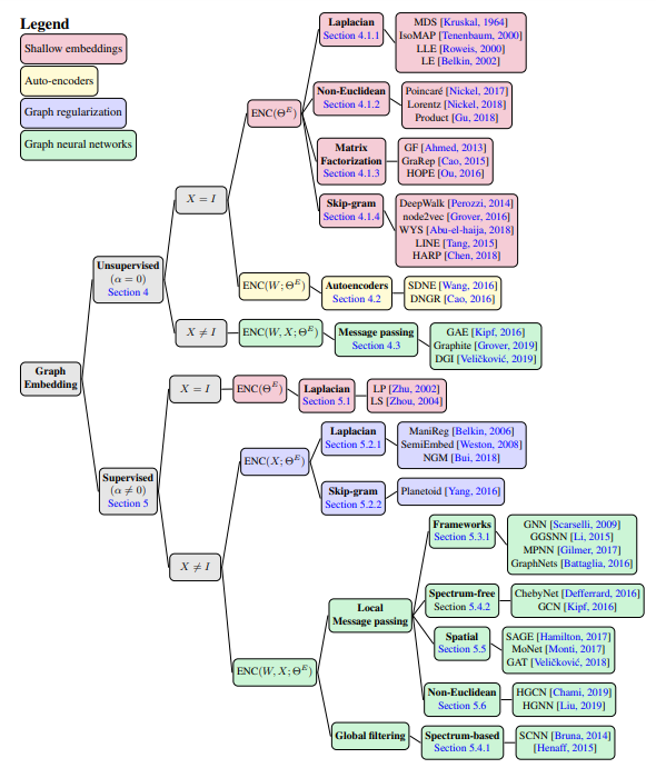
The hierarchical structure of the different unsupervised embedding algorithms

note

It is important to highlight the main role that these algorithms play when we try to solve a machine learning problem on a graph. They can be used passively in order to transform a graph into a feature vector suitable for a classical machine learning algorithm or for data visualization tasks. But they can also be used actively during the learning process, where the machine learning algorithm finds a compact and meaningful solution to a specific problem.

Shallow embedding methods

These methods are able to learn and return only the embedding values for the learned input data. Generally speaking, all the unsupervised embedding algorithms based on matrix factorization use the same principle. They all factorize an input graph expressed as a matrix in different components (commonly knows as matrix factorization). The main difference between each method lies in the loss function used during the optimization process. Indeed, different loss functions allow creating an embedding space that emphasizes specific properties of the input graph.

Graph factorization

The GF algorithm was one of the first models to reach good computational performance in order to perform the node embedding of a given graph. The loss function used in this method was mainly designed to improve GF performances and scalability. Indeed, the solution generated by this method could be noisy. Moreover, it should be noted, by looking at its matrix factorization formulation, that GF performs a strong symmetric factorization. This property is particularly suitable for undirected graphs, where the adjacency matrix is symmetric, but could be a potential limitation for undirected graphs.

Graph autoencoding methods

Network embedding is an important method to learn low-dimensional representations of vertexes in networks, aiming to capture and preserve the network structure. Almost all the existing network embedding methods adopt shallow models. However, since the underlying network structure is complex, shallow models cannot capture the highly non-linear network structure, resulting in sub-optimal network representations. Therefore, how to find a method that is able to effectively capture the highly non-linear network structure and preserve the global and local structure is an open yet important problem.

Autoencoders are an extremely powerful tool that can effectively help data scientists to deal with high-dimensional datasets. Although first presented around 30 years ago, in recent years, autoencoders have become more and more widespread in conjunction with the general rise of neural network-based algorithms. Besides allowing us to compact sparse representations, they can also be at the base of generative models, representing the first inception of the famous Generative Adversarial Network (GAN), which is, using the words of Geoffrey Hinton: "The most interesting idea in the last 10 years in machine learning". An autoencoder is a neural network where the inputs and outputs are basically the same, but that is characterized by a small number of units in the hidden layer. Loosely speaking, it is a neural network that is trained to reconstruct its inputs using a significantly lower number of variables and/or degree of freedom.

Different from other techniques such as Principal Component Analysis (PCA) and matrix factorization, autoencoders can learn non-linear transformation thanks to the non-linear activation functions of their neurons. The encoder-decoder structure is then trained to minimize the ability of the full network to reconstruct the input. In order to completely specify an autoencoder, we need a loss function. The error between the inputs and the outputs can be computed using different metrics and indeed the choice of the correct form for the "reconstruction" error is a critical point when building an autoencoder. Some common choices for the loss functions that measure the reconstruction error are mean square error, mean absolute error, cross-entropy, and KL divergence.

Graph autoencoding methods do not simply learn how to map the input graphs in vectors; they learn a more general mapping function, capable of also generating the embedding vector for unseen instances. When applying autoencoders to graph structures, the input and output of the network should be a graph representation, as, for instance, the adjacency matrix. The reconstruction loss could then be defined as the Frobenius norm of the difference between the input and output matrices. However, when applying autoencoders to such graph structures and adjacency matrices, two critical issues arise:

• Whereas the presence of links indicates a relation or similarity between two vertices, their absence does not generally indicate a dissimilarity between vertices.
• The adjacency matrix is extremely sparse and therefore the model will naturally tend to predict a 0 rather than a positive value.

To address such peculiarities of graph structures, when defining the reconstruction loss, we need to penalize more errors done for the non-zero elements rather than that for zero elements.

Although very powerful, these graph autoencoders encounter some issues when dealing with large graphs. For these cases, the input of our autoencoder is one row of the adjacency matrix that has as many elements as the nodes in the network. In large networks, this size can easily be of the order of millions or tens of millions.

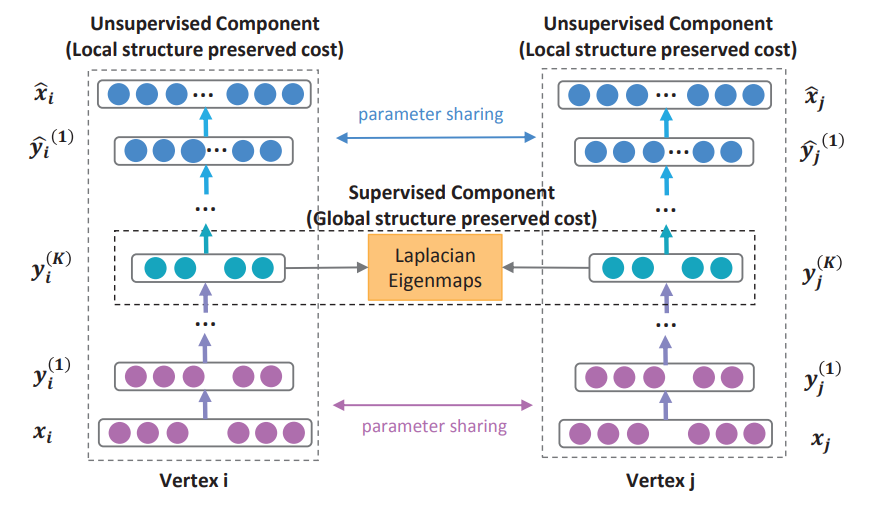
Structural Deep Network Embedding

Wang et. al. proposed a Structural Deep Network Embedding method, namely SDNE. More specifically, they first built a semi-supervised deep model, which has multiple layers of non-linear functions, thereby being able to capture the highly non-linear network structure. Then they exploited the first-order and second-order proximity jointly to preserve the network structure. The second-order proximity is used by the unsupervised component to capture the global network structure. While the first-order proximity is used as the supervised information in the supervised component to preserve the local network structure. By jointly optimizing them in the semi-supervised deep model, this method preserves both the local and global network structure and is robust to sparse networks.

Graph neural networks

GNNs are deep learning methods that work on graph-structured data. This family of methods is also known as geometric deep learning and is gaining increasing interest in a variety of applications, including social network analysis and computer graphics. The original formulation of GNN was proposed by Scarselli et al. back in 2009. It relies on the fact that each node can be described by its features and its neighborhood. Information coming from the neighborhood (which represents the concept of locality in the graph domain) can be aggregated and used to compute more complex and high-level features.

Starting from this first idea, several attempts have been made in recent years to re-address the problem of learning from graph data. In particular, variants of the previously described GNN have been proposed, with the aim of improving its representation learning capability. Some of them are specifically designed to process specific types of graphs (direct, indirect, weighted, unweighted, static, dynamic, and so on). Also, several modifications have been proposed for the propagation step (convolution, gate mechanisms, attention mechanisms, and skip connections, among others), with the aim of improving representation at different levels. Also, different training methods have been proposed to improve learning.

Graph Convolutional Neural Network (GCN)-based encoders are one of the most diffused variants of GNN for unsupervised learning. GCNs are GNN models inspired by many of the basic ideas behind CNN. Filter parameters are typically shared over all locations in the graph and several layers are concatenated to form a deep network.

There are essentially two types of convolutional operations for graph data, namely spectral approaches and non-spectral (spatial) approaches. The first, as the name suggests, defines convolution in the spectral domain (that is, decomposing graphs in a combination of simpler elements). Spatial convolution formulates the convolution as aggregating feature information from neighbors.

Spectral graph convolution

Spectral approaches are related to spectral graph theory, the study of the characteristics of a graph in relation to the characteristic polynomial, eigenvalues, and eigenvectors of the matrices associated with the graph. The convolution operation is defined as the multiplication of a signal (node features) by a kernel. In more detail, it is defined in the Fourier domain by determining the eigendecomposition of the graph Laplacian (think about the graph Laplacian as an adjacency matrix normalized in a special way).

Spectral graph convolution methods have achieved noteworthy results in many domains. However, they present some drawbacks. Consider, for example, a very big graph with billions of nodes: a spectral approach requires the graph to be processed simultaneously, which can be impractical from a computational point of view.

Furthermore, spectral convolution often assumes a fixed graph, leading to poor generalization capabilities on new, different graphs. To overcome these issues, spatial graph convolution represents an interesting alternative.

Spatial graph convolution

Spatial graph convolutional networks perform the operations directly on the graph by aggregating information from spatially close neighbors. Spatial convolution has many advantages: weights can be easily shared across a different location of the graph, leading to a good generalization capability on different graphs. Furthermore, the computation can be done by considering subsets of nodes instead of the entire graph, potentially improving computational efficiency.

GraphSAGE is one of the algorithms that implement spatial convolution. One of the main characteristics is its ability to scale over various types of networks. We can think of GraphSAGE as composed of three steps:

1. Neighborhood sampling: For each node in a graph, the first step is to find its k-neighborhood, where k is defined by the user for determining how many hops to consider (neighbors of neighbors).
2. Aggregation: The second step is to aggregate, for each node, the node features describing the respective neighborhood. Various types of aggregation can be performed, including average, pooling (for example, taking the best feature according to certain criteria), or an even more complicated operation, such as using recurrent units (such as LSTM).
3. Prediction: Each node is equipped with a simple neural network that learns how to perform predictions based on the aggregated features from the neighbors.

GraphSAGE is often used in supervised settings. However, by adopting strategies such as using a similarity function as the target distance, it can also be effective for learning embedding without explicitly supervising the task.

Taxonomy

General design pipeline of graph embedding-based recommendation

A general design pipeline of graph embedding-based recommendation. source.