Transformers
The old, obsolete, 1980 architecture of Recurrent Neural Networks(RNNs) including the LSTMs were simply not producing good results anymore. In less than two years, transformer models wiped RNNs off the map and even outperformed human baselines for many tasks.
Here’s what the transformer block looks like in PyTorch:
class TransformerBlock(nn.Module):
  def __init__(self, k, heads):
    super().__init__()

    self.attention = SelfAttention(k, heads=heads)

    self.norm1 = nn.LayerNorm(k)
    self.norm2 = nn.LayerNorm(k)

    self.ff = nn.Sequential(
      nn.Linear(k, 4 * k),
      nn.ReLU(),
      nn.Linear(4 * k, k))

  def forward(self, x):
    attended = self.attention(x)
    x = self.norm1(attended + x)

    fedforward = self.ff(x)
    return self.norm2(fedforward + x)
Normalization and residual connections are standard tricks used to help deep neural networks train faster and more accurately. The layer normalization is applied over the embedding dimension only.
That is, the block applies, in sequence: a self attention layer, layer normalization, a feed forward layer (a single MLP applied independently to each vector), and another layer normalization. Residual connections are added around both, before the normalization. The order of the various components is not set in stone; the important thing is to combine self-attention with a local feedforward, and to add normalization and residual connections.
The transformer block
- Multi-head attention
- Scaling the dot product
- Queries, keys and values
The actual self-attention used in modern transformers relies on three additional tricks.
Additional tricks
import torch
import torch.nn.functional as F

# assume we have some tensor x with size (b, t, k)
x = ...

raw_weights = torch.bmm(x, x.transpose(1, 2))
# - torch.bmm is a batched matrix multiplication. It
#   applies matrix multiplication over batches of
#   matrices.

weights = F.softmax(raw_weights, dim=2)

y = torch.bmm(weights, x)
We’ll represent the input, a sequence of t vectors of dimension k as a t by k matrix 𝐗. Including a minibatch dimension b, gives us an input tensor of size (b,t,k). The set of all raw dot products w′ij forms a matrix, which we can compute simply by multiplying 𝐗 by its transpose. Then, to turn the raw weights w′ij into positive values that sum to one, we apply a row-wise softmax. Finally, to compute the output sequence, we just multiply the weight matrix by 𝐗. This results in a batch of output matrices 𝐘 of size (b, t, k) whose rows are weighted sums over the rows of 𝐗. That’s all. Two matrix multiplications and one softmax gives us a basic self-attention.
In Pytorch: basic self-attention
Let's understand with RecSys analogy. The tokens are both users and items. In movie recommenders e.g., to know a user's interest in different movies, we take a dot product of his embedding vector with movies' embedding vectors. Here in self-attention, we take a dot of the given token with all other tokens to know how much the given token is connected to other tokens.
In effect, there are five processes we need to understand to implement this model:
- Embedding the inputs
- The Positional Encodings
- Creating Masks
- The Multi-Head Attention layer
- The Feed-Forward layer
Embedding
Embedding is handled simply in PyTorch:
class Embedder(nn.Module):
    def __init__(self, vocab_size, d_model):
        super().__init__()
        self.embed = nn.Embedding(vocab_size, d_model)
    def forward(self, x):
        return self.embed(x)
When each word is fed into the network, this code will perform a look-up and retrieve its embedding vector. These vectors will then be learnt as a parameters by the model, adjusted with each iteration of gradient descent.
Giving our words context: The Positional Encodings
In order for the model to make sense of a sentence, it needs to know two things about each word: what does the word mean? And what is its position in the sentence?
The embedding vector for each word will learn the meaning, so now we need to input something that tells the network about the word’s position.
Vasmani et al answered this problem by using these functions to create a constant of position-specific values:
This constant is a 2d matrix. refers to the order in the sentence, and i $refers to the position along the embedding vector dimension. Each value in the $pos/i matrix is then worked out using the equations above.
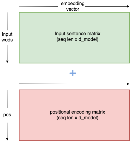
The positional encoding matrix is a constant whose values are defined by the above equations. When added to the embedding matrix, each word embedding is altered in a way specific to its position.
An intuitive way of coding our Positional Encoder looks like this:
class PositionalEncoder(nn.Module):
    def __init__(self, d_model, max_seq_len = 80):
        super().__init__()
        self.d_model = d_model

        # create constant 'pe' matrix with values dependant on
        # pos and i
        pe = torch.zeros(max_seq_len, d_model)
        for pos in range(max_seq_len):
            for i in range(0, d_model, 2):
                pe[pos, i] = \
                math.sin(pos / (10000 ** ((2 * i)/d_model)))
                pe[pos, i + 1] = \
                math.cos(pos / (10000 ** ((2 * (i + 1))/d_model)))

        pe = pe.unsqueeze(0)
        self.register_buffer('pe', pe)


    def forward(self, x):
        # make embeddings relatively larger
        x = x * math.sqrt(self.d_model)
        #add constant to embedding
        seq_len = x.size(1)
        x = x + Variable(self.pe[:,:seq_len], \
        requires_grad=False).cuda()
        return x
The above module lets us add the positional encoding to the embedding vector, providing information about structure to the model.
Creating Our Masks
Masking plays an important role in the transformer. It serves two purposes:
- In the encoder and decoder: To zero attention outputs wherever there is just padding in the input sentences.
- In the decoder: To prevent the decoder ‘peaking’ ahead at the rest of the translated sentence when predicting the next word.
Creating the mask for the input is simple:
batch = next(iter(train_iter))
input_seq = batch.English.transpose(0,1)
input_pad = EN_TEXT.vocab.stoi['<pad>']# creates mask with 0s wherever there is padding in the input
input_msk = (input_seq != input_pad).unsqueeze(1)
For the target_seq we do the same, but then create an additional step:
# create mask as beforetarget_seq = batch.French.transpose(0,1)
target_pad = FR_TEXT.vocab.stoi['<pad>']
target_msk = (target_seq != target_pad).unsqueeze(1)size = target_seq.size(1) # get seq_len for matrixnopeak_mask= np.triu(np.ones(1, size, size),
k=1).astype('uint8')
nopeak_mask = Variable(torch.from_numpy(nopeak_mask)== 0)target_msk = target_msk & nopeak_mask
Multi-Headed Attention
Once we have our embedded values (with positional encodings) and our masks, we can start building the layers of our model.
Here is an overview of the multi-headed attention layer:
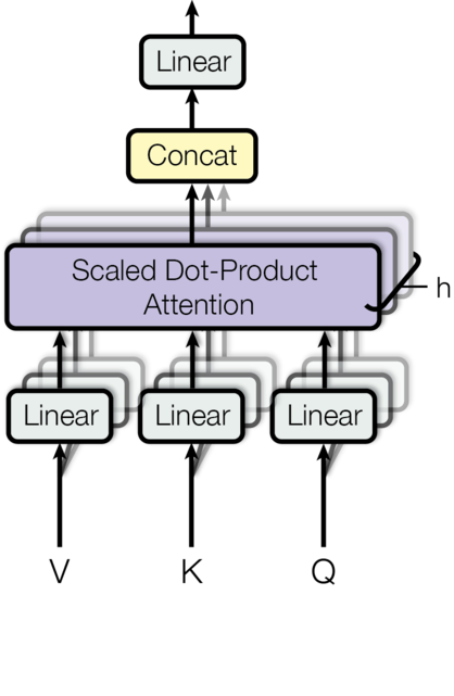
Multi-headed attention layer, each input is split into multiple heads which allows the network to simultaneously attend to different subsections of each embedding.
A scaled dot-product attention mechanism is very similar to a self-attention (dot-product) mechanism except it uses a scaling factor. The multi-head part, on the other hand, ensures the model is capable of looking at various aspects of input at all levels. Transformer models attend to encoder annotations and the hidden values from past layers. The architecture of the Transformer model does not have a recurrent step-by-step flow; instead, it uses positional encoding in order to have information about the position of each token in the input sequence. The concatenated values of the embeddings (randomly initialized) and the fixed values of positional encoding are the input fed into the layers in the first encoder part and are propagated through the architecture.
In the case of the Encoder, V, K and G will simply be identical copies of the embedding vector (plus positional encoding). They will have the dimensions Batch_size seq_len d_model.
In multi-head attention we split the embedding vector into N heads, so they will then have the dimensions
This final dimension we will refer to as .
Let’s see the code for the decoder module:
class MultiHeadAttention(nn.Module):
    def __init__(self, heads, d_model, dropout = 0.1):
        super().__init__()

        self.d_model = d_model
        self.d_k = d_model // heads
        self.h = heads

        self.q_linear = nn.Linear(d_model, d_model)
        self.v_linear = nn.Linear(d_model, d_model)
        self.k_linear = nn.Linear(d_model, d_model)
        self.dropout = nn.Dropout(dropout)
        self.out = nn.Linear(d_model, d_model)

    def forward(self, q, k, v, mask=None):

        bs = q.size(0)

        # perform linear operation and split into h heads

        k = self.k_linear(k).view(bs, -1, self.h, self.d_k)
        q = self.q_linear(q).view(bs, -1, self.h, self.d_k)
        v = self.v_linear(v).view(bs, -1, self.h, self.d_k)

        # transpose to get dimensions bs * h * sl * d_model

        k = k.transpose(1,2)
        q = q.transpose(1,2)
        v = v.transpose(1,2)
                # calculate attention using function we will define next
        scores = attention(q, k, v, self.d_k, mask, self.dropout)

        # concatenate heads and put through final linear layer
        concat = scores.transpose(1,2).contiguous()\
        .view(bs, -1, self.d_model)

        output = self.out(concat)

        return output
Calculating Attention
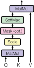
Initially we must multiply Q by the transpose of K. This is then ‘scaled’ by dividing the output by the square root of . Before we perform Softmax, we apply our mask and hence reduce values where the input is padding (or in the decoder, also where the input is ahead of the current word). Finally, the last step is doing a dot product between the result so far and V.
Here is the code for the attention function:
def attention(q, k, v, d_k, mask=None, dropout=None):
    scores = torch.matmul(q, k.transpose(-2, -1)) /  math.sqrt(d_k)

        if mask is not None:
        mask = mask.unsqueeze(1)
        scores = scores.masked_fill(mask == 0, -1e9)

        scores = F.softmax(scores, dim=-1)

    if dropout is not None:
        scores = dropout(scores)

    output = torch.matmul(scores, v)
    return output
In PyTorch, it looks like this:
from torch import Tensor
import torch.nn.functional as f

def scaled_dot_product_attention(query: Tensor, key: Tensor, value: Tensor) -> Tensor:
    temp = query.bmm(key.transpose(1, 2))
    scale = query.size(-1) ** 0.5
    softmax = f.softmax(temp / scale, dim=-1)
    return softmax.bmm(value)
Note that MatMul operations are translated to torch.bmm in PyTorch. That’s because Q, K, and V (query, key, and value arrays) are batches of matrices, each with shape (batch_size, sequence_length, num_features). Batch matrix multiplication is only performed over the last two dimensions.
The attention head will then become:
import torch
from torch import nn

class AttentionHead(nn.Module):
    def __init__(self, dim_in: int, dim_k: int, dim_v: int):
        super().__init__()
        self.q = nn.Linear(dim_in, dim_k)
        self.k = nn.Linear(dim_in, dim_k)
        self.v = nn.Linear(dim_in, dim_v)

    def forward(self, query: Tensor, key: Tensor, value: Tensor) -> Tensor:
        return scaled_dot_product_attention(self.q(query), self.k(key), self.v(value))
Now, it’s very easy to build the multi-head attention layer. Just combine num_heads different attention heads and a Linear layer for the output.
class MultiHeadAttention(nn.Module):
    def __init__(self, num_heads: int, dim_in: int, dim_k: int, dim_v: int):
        super().__init__()
        self.heads = nn.ModuleList(
            [AttentionHead(dim_in, dim_k, dim_v) for _ in range(num_heads)]
        )
        self.linear = nn.Linear(num_heads * dim_v, dim_in)

    def forward(self, query: Tensor, key: Tensor, value: Tensor) -> Tensor:
        return self.linear(
            torch.cat([h(query, key, value) for h in self.heads], dim=-1)
        )
Let’s pause again to examine what’s going on in the MultiHeadAttention layer. Each attention head computes its own query, key, and value arrays, and then applies scaled dot-product attention. Conceptually, this means each head can attend to a different part of the input sequence, independent of the others. Increasing the number of attention heads allows us to “pay attention” to more parts of the sequence at once, which makes the model more powerful.
The Feed-Forward Network
This layer just consists of two linear operations, with a relu and dropout operation in between them.
class FeedForward(nn.Module):
    def __init__(self, d_model, d_ff=2048, dropout = 0.1):
        super().__init__()
        # We set d_ff as a default to 2048
        self.linear_1 = nn.Linear(d_model, d_ff)
        self.dropout = nn.Dropout(dropout)
        self.linear_2 = nn.Linear(d_ff, d_model)
    def forward(self, x):
        x = self.dropout(F.relu(self.linear_1(x)))
        x = self.linear_2(x)
        return x
The feed-forward layer simply deepens our network, employing linear layers to analyze patterns in the attention layers output.
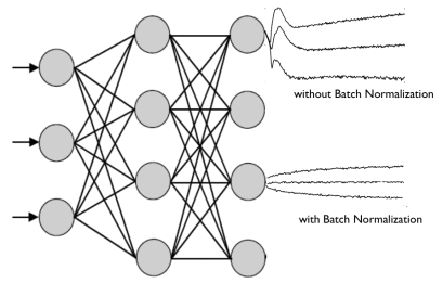
One Last Thing : Normalization
Normalisation is highly important in deep neural networks. It prevents the range of values in the layers changing too much, meaning the model trains faster and has better ability to generalise.
We will be normalizing our results between each layer in the encoder/decoder, so before building our model let’s define that function:
class Norm(nn.Module):
    def __init__(self, d_model, eps = 1e-6):
        super().__init__()

        self.size = d_model
        # create two learnable parameters to calibrate normalisation
        self.alpha = nn.Parameter(torch.ones(self.size))
        self.bias = nn.Parameter(torch.zeros(self.size))
        self.eps = eps
    def forward(self, x):
        norm = self.alpha * (x - x.mean(dim=-1, keepdim=True)) \
        / (x.std(dim=-1, keepdim=True) + self.eps) + self.bias
        return norm
Putting it all together!
Let’s have another look at the over-all architecture and start building:
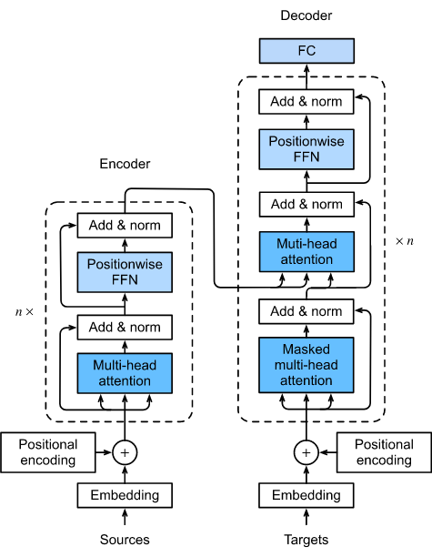
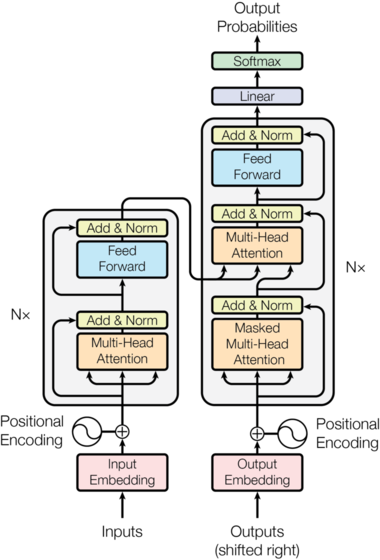
One last Variable: If you look at the diagram closely you can see a ‘Nx’ next to the encoder and decoder architectures. In reality, the encoder and decoder in the diagram above represent one layer of an encoder and one of the decoder. N is the variable for the number of layers there will be. Eg. if N=6, the data goes through six encoder layers (with the architecture seen above), then these outputs are passed to the decoder which also consists of six repeating decoder layers.
We will now build EncoderLayer and DecoderLayer modules with the architecture shown in the model above. Then when we build the encoder and decoder we can define how many of these layers to have.
# build an encoder layer with one multi-head attention layer and one # feed-forward layer
class EncoderLayer(nn.Module):
    def __init__(self, d_model, heads, dropout = 0.1):
        super().__init__()
        self.norm_1 = Norm(d_model)
        self.norm_2 = Norm(d_model)
        self.attn = MultiHeadAttention(heads, d_model)
        self.ff = FeedForward(d_model)
        self.dropout_1 = nn.Dropout(dropout)
        self.dropout_2 = nn.Dropout(dropout)

    def forward(self, x, mask):
        x2 = self.norm_1(x)
        x = x + self.dropout_1(self.attn(x2,x2,x2,mask))
        x2 = self.norm_2(x)
        x = x + self.dropout_2(self.ff(x2))
        return x

# build a decoder layer with two multi-head attention layers and
# one feed-forward layer
class DecoderLayer(nn.Module):
    def __init__(self, d_model, heads, dropout=0.1):
        super().__init__()
        self.norm_1 = Norm(d_model)
        self.norm_2 = Norm(d_model)
        self.norm_3 = Norm(d_model)

        self.dropout_1 = nn.Dropout(dropout)
        self.dropout_2 = nn.Dropout(dropout)
        self.dropout_3 = nn.Dropout(dropout)

        self.attn_1 = MultiHeadAttention(heads, d_model)
        self.attn_2 = MultiHeadAttention(heads, d_model)
        self.ff = FeedForward(d_model).cuda()

        def forward(self, x, e_outputs, src_mask, trg_mask):
        x2 = self.norm_1(x)
        x = x + self.dropout_1(self.attn_1(x2, x2, x2, trg_mask))
        x2 = self.norm_2(x)
        x = x + self.dropout_2(self.attn_2(x2, e_outputs, e_outputs,
        src_mask))
        x2 = self.norm_3(x)
        x = x + self.dropout_3(self.ff(x2))
        return x

        # We can then build a convenient cloning function that can generate multiple layers:
        def get_clones(module, N):
            return nn.ModuleList([copy.deepcopy(module) for i in range(N)])
We’re now ready to build the encoder and decoder:
class Encoder(nn.Module):
    def __init__(self, vocab_size, d_model, N, heads):
        super().__init__()
        self.N = N
        self.embed = Embedder(vocab_size, d_model)
        self.pe = PositionalEncoder(d_model)
        self.layers = get_clones(EncoderLayer(d_model, heads), N)
        self.norm = Norm(d_model)
    def forward(self, src, mask):
        x = self.embed(src)
        x = self.pe(x)
        for i in range(N):
            x = self.layers[i](x, mask)
        return self.norm(x)

class Decoder(nn.Module):
    def __init__(self, vocab_size, d_model, N, heads):
        super().__init__()
        self.N = N
        self.embed = Embedder(vocab_size, d_model)
        self.pe = PositionalEncoder(d_model)
        self.layers = get_clones(DecoderLayer(d_model, heads), N)
        self.norm = Norm(d_model)
    def forward(self, trg, e_outputs, src_mask, trg_mask):
        x = self.embed(trg)
        x = self.pe(x)
        for i in range(self.N):
            x = self.layers[i](x, e_outputs, src_mask, trg_mask)
        return self.norm(x)
And finally… The transformer!
class Transformer(nn.Module):
    def __init__(self, src_vocab, trg_vocab, d_model, N, heads):
        super().__init__()
        self.encoder = Encoder(src_vocab, d_model, N, heads)
        self.decoder = Decoder(trg_vocab, d_model, N, heads)
        self.out = nn.Linear(d_model, trg_vocab)
    def forward(self, src, trg, src_mask, trg_mask):
        e_outputs = self.encoder(src, src_mask)
        d_output = self.decoder(trg, e_outputs, src_mask, trg_mask)
        output = self.out(d_output)
        return output
# we don't perform softmax on the output as this will be handled
# automatically by our loss function
The original Transformer model is a stack of 6 layers. The output of layer l is the input of layer l+1 until the final prediction is reached. There is a 6-layer encoder stack on the left and a 6-layer decoder stack on the right:
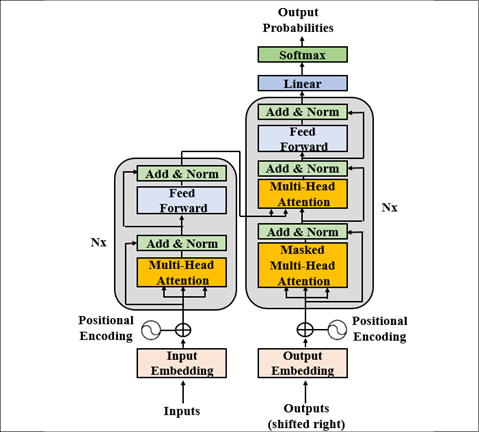
The architecture of the Transformer
On the left, the inputs enter the encoder side of the Transformer through an attention sub-layer and FeedForward Network (FFN) sub-layer. On the right, the target outputs go into the decoder side of the Transformer through two attention sub-layers and an FFN sub-layer. We immediately notice that there is no RNN, LSTM, or CNN. Recurrence has been abandoned. Attention has replaced recurrence, which requires an increasing number of operations as the distance between two words increases.
The attention mechanism is a "word-to-word" operation. The attention mechanism will find how each word is related to all other words in a sequence, including the word being analyzed itself.